Ververica Platform 2.3: Getting Started with Flink SQL on Ververica Platform

Flink SQL is one of the three main programming interfaces of Apache Flink. ; It is declarative and, because the community kept the syntax inline with the SQL standard, anyone who knows traditional SQL will feel familiar within minutes. Flink SQL has managed to unify batch and stream processing. This means that you can run the same query on a bounded table (a data set) as a batch job or an unbounded table (a stream of data) as a long-running stream processing application and — given the same input — the resulting table will be identical.

Two weeks ago we released Ververica Platform 2.3 ;which brought development, operations, and management capabilities for Flink SQL to Ververica Platform. In this blog post, I would like to walk you through a simple analytics use case of Flink SQL on Ververica Platform. We will use Flink SQL to read temperature measurements from an Apache Kafka topic, continuously derive statistics, and write these statistics back to a different Kafka topic. ;

Reading From Kafka

Flink SQL operates on tables that can be read from and written to. In contrast to a traditional database or data warehouse, Apache Flink does not store the tables itself. Tables are always backed by an external system. So, to read temperature measurements from Kafka we need to define a table over our input topic.

As illustrated in Figure 1, we choose a template for a new table via + in the Schema Explorer and choose “Kafka” and “Confluent Avro” format, because that is where our measurement data resides.

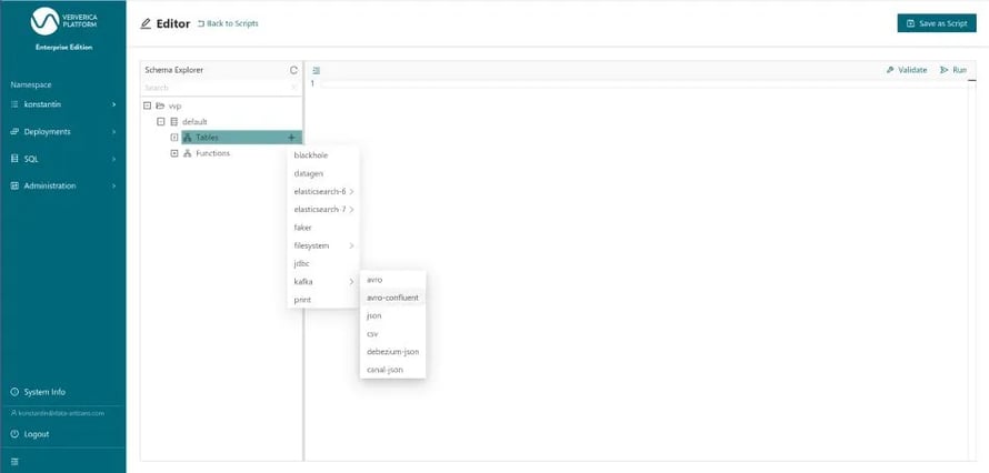Figure 1: Selecting a CREATE TABLE template for “kafka” with “confluent-avro” format

Then we need to fill in the template. Besides the name temperature_measurements, we first supply the schema of the table. The schema supplied here will be the one used to deserialize the Avro records read from Kafka. As such, it needs to be compatible with the schema that these records have been serialized with, which is fetched from the schema registry when reading the table. Second, you use the table options to configure the external system that this table is stored in. Since we are using Kafka with Confluent’s Avro this entails configuring Kafka bootstrap servers, the Kafka topic and the connection to the schema registry. ;

Finally, we provide a watermark for the measurement_time column. Defining a watermark for a column informs Apache Flink about the expected delay and out-of-orderness in which rows are added to this table. Concretely, WATERMARK FOR measurement_time AS measument_time - INTERVAL ‘15’ SECONDS tells the framework that measurements might come up to 15 seconds out-of-order with respect to the measurement_time. Without a WATERMARK definition, a TIMESTAMP column cannot be used for time-based operations like event time windowing or sorting an unbounded table by time.

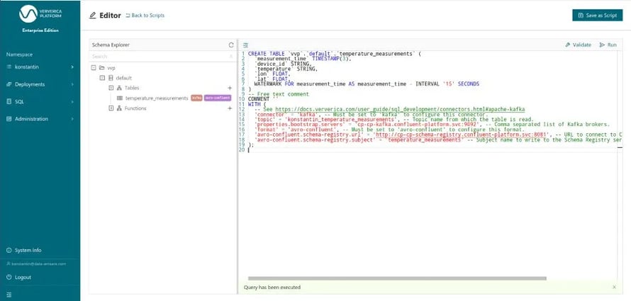Figure 2: Executing the CREATE TABLE statement for temperature_measurements

After executing the CREATE TABLE statement the definition of the temperatue_measurements table is durably stored in the vvp catalog and will be available to other users of that platform namespace going forward as well.

Now, we can run queries on that table. To start with, let us simply take a look at rows of that Kafka-backed table by running SELECT * FROM temperature_measurements. Thereby, we are also making sure that the table has been properly configured before building more complicated queries.

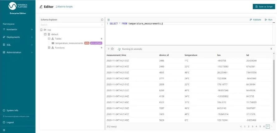Figure 3: Executing a SELECT query over a Kafka-backed table form the editor

Being able to query any Flink table from the browser like this is already pretty cool. Particularly because this provides a common interface to query data distributed over various systems like Kafka, ElasticSearch, Hive, MySQL, and more.

Developing our Query

Next, we would like to continuously derive statistics about the measurement records as they come in. Specifically, we would like to derive the average temperature per minute based on the measurement_time.

The temperature column is currently a STRING column and includes the unit °C. In order to take the average, we need to strip the unit and cast the type to a FLOAT. We do this by using two different built-in functions REGEXP_ETRACT and CAST.

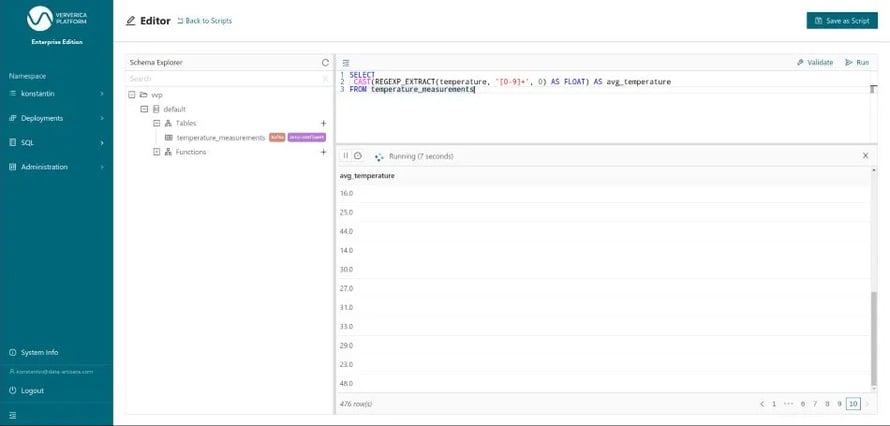Figure 4: Transforming the temperature column from STRING to FLOAT

To compute the average temperature over one minute windows, we use a so called GROUP BY window aggregation with a tumbling window. Tumbling windows have a fixed-length and are non-overlapping. We use TUMBLE to group the rows/records, TUMBLE_ROWTIME to extract the timestamp of the window for the final results and AVG to compute the actual average. So, the final statement will look like this:

SELECT
 TUMBLE_ROWTIME(measurement_time, INTERVAL '1' MINUTE) AS window_time,
 AVG(CAST(REGEXP_EXTRACT(temperature, '[0-9]+', 0) AS FLOAT)) AS avg_temperature
FROM temperature_measurements
GROUP BY
 TUMBLE(measurement_time, INTERVAL '1' MINUTE)

When you run this statement (Figure 5) you’ll see one result row about every minute, because the result rows are only written out once the window end time has passed and the window is closed.

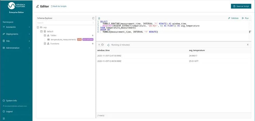Figure 5: Running our final query from the editor

Writing Back to Kafka

Since we have now established that our query is doing what it should be, we need to write the results into another table. Only by doing so, the results can be consumed by downstream applications. You can also think about it as creating a materialized view based on the temperature_measurement table that is continuously maintained by Apache Flink. We will call the result table average_temperatures and again store it in a Kafka topic with Confluent’s Avro format. Figure 7 shows the corresponding CREATE TABLE statement. Fortunately, the schema and the table name have automatically been templated by the platform based on the INSERT INTO statement below it, so that we only need to provide the missing table options like the Kafka topic.

Figure 6: Executing (“Run Selection”) the CREATE TABLE statement for the result table average_temperatures

Now, we can “Run” the final INSERT INTO statement. As outlined above an INSERT INTO statement based on an unbounded table is a continuous query, similar to the definition of a materialized view. Therefore, the platform now asks us whether we would like to create a Deployment for this query. A Deployment is Ververica Platform’s abstraction for a long running service or application. ;

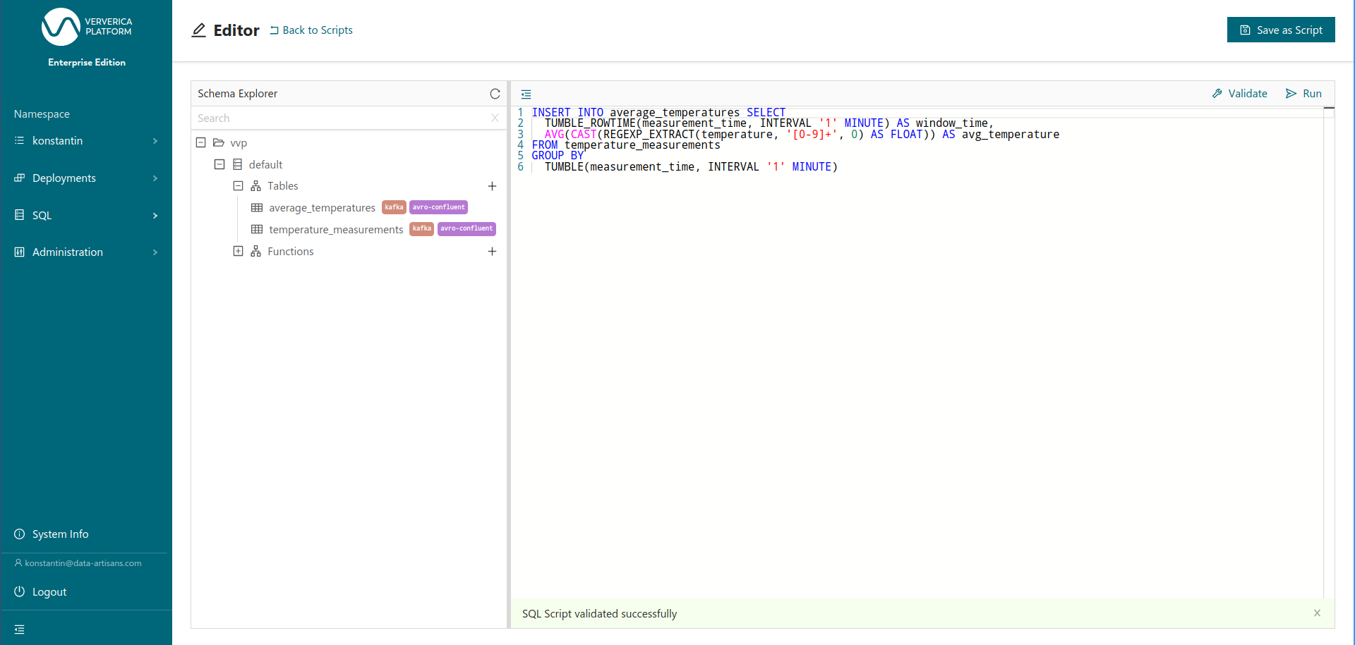Figure 7: Validating the final query: a tumbling window aggregation on temperature_measurements

We confirm and finalize the Deployment creation form (Figure 8) by giving the Deployment a name and hitting CREATE SQL Deployment.

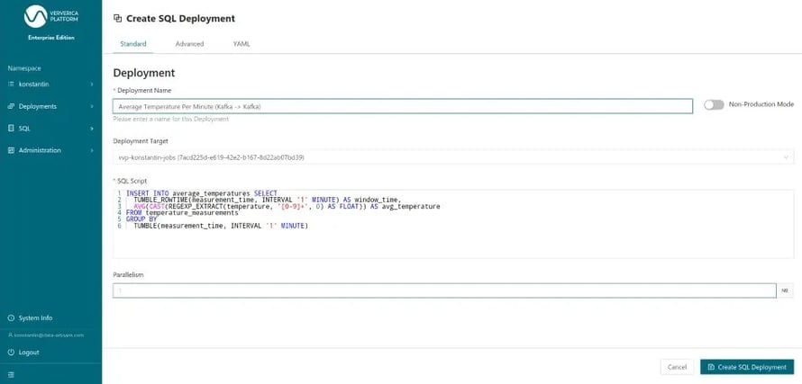Figure 8: Submitting the query as a long-running Deployment

Afterward, we can return to the editor and — once the Deployment is running — query the average_temperatures table directly. Because we only need to query the existing table instead of executing the underlying query, data is now available within seconds (Figure 10).

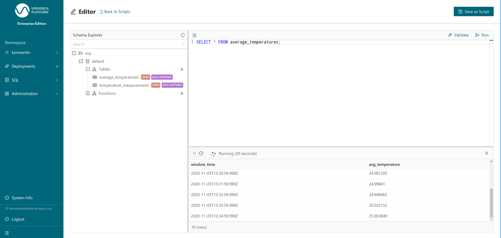Figure 10: Querying the result table average_temepratures

And that’s all for now. This is all you need to build and deploy a highly scalable, flexible data pipeline with Flink SQL and Ververica Platform, but of course, there is still a lot to cover in the upcoming weeks: user-defined functions, different connectors & catalogs, pattern matching, query management,... If you are interested in learning more, I recommend diving in hands-on with our self-contained getting started guide.