Streamhouse: Data Processing Patterns

Introduction

In October, at Flink Forward 2023, Streamhouse was officially introduced by Jing Ge, Head of Engineering at Ververica. In his keynote, Jing highlighted the need for Streamhouse, including how it sits as a layer between real-time stream processing and Lakehouse architectures, and discussed the business value it provides.

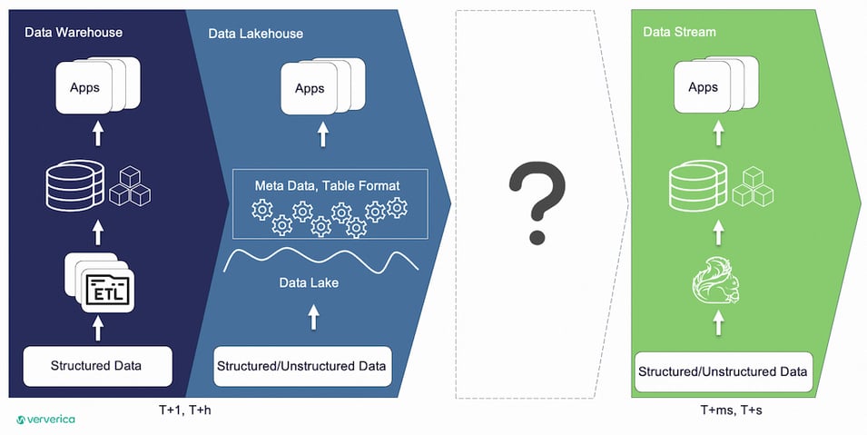
The three musketeers of Streamhouse architecture were also introduced: Apache Flink®️, Flink CDC, and Apache Paimon. You can also find an introduction in Apache Paimon: The Streaming Lakehouse.

Apache Paimon was created as a Lakehouse table format, but it is much more than that.

It extends Apache Flink’s capabilities on the datalake and allows developers to truly leverage stream processing on the datalake. In this blog post, we will try to better understand what this means in practice by taking a streaming patterns-based approach.

Business Layers of Lakehouse

Before we dive into the different stream processing patterns, let’s make a quick recap of Lakehouse Architecture.

Lakehouse combines the structured nature of data warehouses with the cheap and durable storage of data lakes. Streamhouse builds on this concept, providing stream processing capabilities when near-real-time results are acceptable by the business.

The following illustration highlights the different business layers that you typically see in a data warehouse, and these can keep updating in near-real time on the data lake.

This brings a few benefits, like reduced engineering maintenance effort, which makes the developer's life easier.

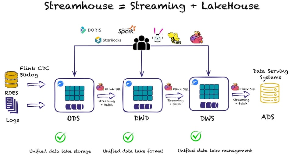
We can observe the following business layers: Operational Data Store (ODS), Data Warehouse Detail (DWD), Data Warehouse Summary (DWS), and Application Data Service (ADS).

ODS

This is typically where the raw, unstructured data gets ingested. The structure of a data table at the ODS layer is the same as the structure of a data table in which the raw data is stored. The ODS layer serves as the staging area for the data warehouse.

DWD

At this layer, data models are built based on the business activities of an enterprise. You can create a fact table that uses the highest granularity level based on the characteristics of a specific business activity. You can duplicate some key attribute fields of dimensions in fact tables and create wide tables based on the data usage habits of the enterprise. You can also associate fact tables with dimension tables as little as possible to improve the usability of fact tables.

DWS

At this layer, data models are built based on specific subject objects that you want to analyze. You can create a general aggregate table based on the metric requirements of upper-layer applications and products.
Some general dimensions can be abstracted at the ODS layer based on preliminary classification and a summary of user behavior. At the DWS layer, you can add multi-granularity aggregate tables on top of general aggregate tables to improve the calculation efficiency

ADS

This layer stores the metric data of products and generates various reports.

Streaming Patterns on the Lake

Pattern 1: Event Deduplication

Event deduplication is about removing duplicate events. Apache Paimon includes two merge engines to support that, i.e. the deduplicate and the first-row merge engines.

-- Deduplicate (also the Default) Merge Engine
CREATE TABLE test (
   key INT,
   field_a INT,
   field_b INT,
   field_c INT,
   field_d INT,
       PRIMARY KEY (key) NOT ENFORCED
) WITH (
   'merge-engine' = 'deduplicate',
   ...
);

-- First-Row Merge Engine
CREATE TABLE test (
   key INT,
   field_a INT,
   field_b INT,
   field_c INT,
   field_d INT,
       PRIMARY KEY (key) NOT ENFORCED
) WITH (
   'merge-engine' = 'first-row',
   'changelog-producer' = 'lookup'
);

• Deduplicate (default): When two events with the same key arrive, only the latest entry is retained.
• First-row: Always retains the first entry around.

Pattern 2: Table Widening

Star schemas are a popular way of normalizing data within a data warehouse. At the center of a star schema is a fact table whose rows contain metrics, measurements, and other facts about the world. Surrounding fact tables are one or more dimension tables that have metadata useful for enriching facts when computing queries.

Similarly, when dealing with streaming data, you might have an append-only stream, (for example, coming from Kafka,) and you want to “widen” this stream with data that live in other sources (one example is Kafka topics).

The way to achieve this would be to run a streaming join which is quite an expensive computation, especially if your tables are large, since the data needs to be stored in state.

Things get even more complicated if we come across data skew, because some keys have way more data than others, resulting in some tasks having to process far bigger workloads than others.

Paimon has done lots of work on this and has introduced the concept of the partial-update merge engine.

Instead of running a streaming join, with the partial-update merge engine, users have the ability to update columns of a record through multiple updates until the record is complete. This is achieved by updating the value fields one by one, using the latest data under the same primary key. However, null values do not overwrite existing non-null values.

For example, suppose Paimon receives three records, with one and three coming from the primary topic, while the second record contains more information we want in order to widen our table:

• <1, 23.0, 10, NULL>
• <1, NULL, NULL, 'This is a book'>
• <1, 25.2, NULL, NULL>

Assuming that the first column is the primary key, the final result would be:

<1, 25.2, 10, 'This is a book'>

The partial-update merge engine also has the concept of sequence groups as we will see next, in order to better control updates and out-of-order events.

Pattern 3: Out-of-Order Event Handling

When dealing with streaming data, we often come across scenarios in which some events arrive late and out of order into our system due to some delay.

Apache Paimon helps address event ordering by allowing users to specify sequence fields. By specifying a sequence field (for example the event timestamp), Paimon knows whether events arrive late and out of order, to better ensure result correctness.

Following is an example of how to specify a sequence field upon table creation.

-- Sequence Fields
CREATE TABLE test (
   pk BIGINT,
   v1 DOUBLE PRECISION,
   V2 BIGING,
   dt TIMESTAMP(3),
       PRIMARY KEY (pk) NOT ENFORCED
) WITH (
   'sequence.field' = 'dt',
   ...
);

As mentioned for the partial update merge engine, Paimon also offers the concept of sequence groups. A sequence field may not solve the “out-of-order” problem of the partial update merge engine with multiple stream updates, because the latest data of another stream may overwrite the sequence field during a multi-stream update.

Sequence groups allow handling events arriving out-of-order during multi-stream updates as each stream can define its own sequence group and define how different columns should be updated.

The following code snippet depicts an example of using the partial update merge engine, along with sequence groups:

-- Sequence Groups
CREATE TABLE test (
   k INT,
   a INT,
   b INT,
   g_1 TIMESTAMP_LTZ(3),
   c INT,
   d INT,
   g_2 TIMESTAMP_LTZ(3),
       PRIMARY KEY (k) NOT ENFORCED
) WITH (
   'merge-engine'='partial-update',
   'changelog-producer'='lookup',
   'fields.g_1.sequence-group'='a,b',
   'fields.g_2.sequence-group'='c,d',
   ...
);


INSERT INTO test
VALUES
   (1, 1, 1, CAST('2023-11-13 10:08:22.001' AS TIMESTAMP(3)), 1, 1, CAST('2023-11-13 10:08:22.001' AS TIMESTAMP(3)));

-- output 1, 1, 1, 2023-11-13 10:08:22.001, 1, 1, 2023-11-13 10:08:22.001
SELECT * FROM test

-- g_2 timestamp is smaller, c, d should not be updated
INSERT INTO test
VALUES
   (1, 2, 2, CAST('2023-11-13 11:08:22.001' AS TIMESTAMP(3)), 2, 2, CAST('2023-11-13 9:08:22.001' AS TIMESTAMP(3)));

-- output 1, 2, 2, 2023-11-13 11:08:22.001, 1, 1, 2023-11-13 10:08:22.001
SELECT * FROM test

-- g_1 timestamp is smaller, a, b should not be updated
INSERT INTO test
VALUES
   (1, 3, 3, CAST('2023-11-13 09:08:22.001' AS TIMESTAMP(3)), 3, 3, CAST('2023-11-13 12:08:22.001' AS TIMESTAMP(3)));

-- output 1, 2, 2, 2023-11-13 11:08:22.001, 3, 3, 2023-11-13 12:08:22.001
SELECT * FROM test;

Pattern 4: Automatic Aggregations

Business layers like the DWS and ADS might require business aggregates or reports to be generated. Paimon helps with that through the aggregation merge engine.

When creating a table using the aggregation merge engine, it allows configuring aggregation functions. These aggregation functions will be applied automatically, every time a new record arrives.

The following code snippet depicts an example of using the aggregation merge engine to create a table that keeps a purchase summary on the ADS layer.

CREATE TABLE `purchase_summary.ads` (
   user_id          STRING NOT NULL,
   user_session     STRING,
   full_name        STRING NOT NULL,
   event_types      STRING,
   num_of_purchases INTEGER,
   products         STRING,
   price_sum        DECIMAL(15,2) NOT NULL,
   min_price        DECIMAL(15,2) NOT NULL,
   max_price        DECIMAL(15,2) NOT NULL,
   PRIMARY KEY (user_session) NOT ENFORCED
) WITH (
   'bucket' = '1',
   'bucket-key' = 'user_session',
   'file.format' = 'parquet',
   'merge-engine' = 'aggregation',
   'changelog-producer' = 'lookup',
   'fields.user_id.aggregate-function'='last_value',
   'fields.full_name.aggregate-function'='last_value',
   'fields.event_types.aggregate-function'='listagg',
   'fields.num_of_purchases.aggregate-function'='sum',
   'fields.products.aggregate-function'='listagg',
   'fields.price_sum.aggregate-function'='sum',
   'fields.max_price.aggregate-function'='max',
   'fields.min_price.aggregate-function'='min'
);

Notice how we can specify different aggregation functions for different column types. For example, we can specify that we want all the event_types to be collected as a list and how for the min, max, and price sum we use the min, max, and sum aggregation functions respectively.

Pattern 5: Message Queue on the Data Lake

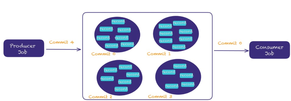
Apache Paimon’s append-only table allows implementing message queue functionality on the data lake.

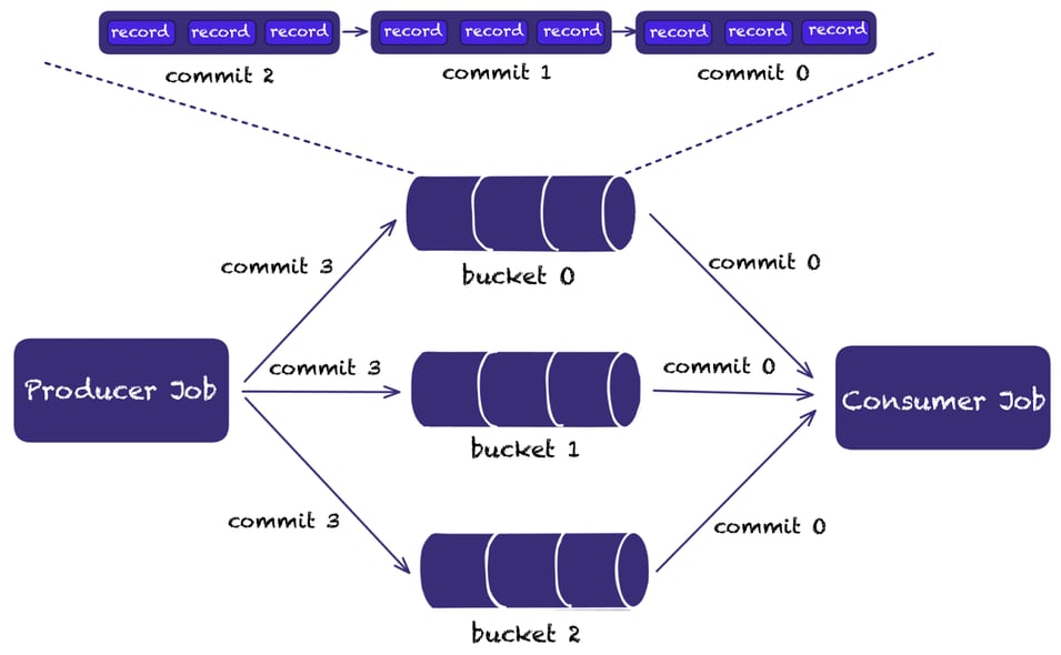
Similar to Kafka’s topics and partitions, Paimon has tables and buckets.

Users can create multiple buckets, and within each bucket, every record is in strict order. Streaming reads will propagate the records downstream in the exact order of writing.

Similar to the partition number in a topic, the bucket number in a table defines the number of parallelism for processing and the user can define a bucket key for splitting the data across multiple buckets.

The following illustration depicts this functionality.

Pattern 6: Data Backfilling and Correction with Time Travel

Another important functionality is querying the state of your tables at different points in time or identifying what changed between different snapshots. This helps with use cases when you want to perform data backfills, identify data corruptions, and restore to previous versions. For example, you might want to analyze the finances of your business across different quarters, identify data that has been corrupted or deleted, or reproduce business reports.

MERGE INTO functionality is also supported if you want to fix errors that might have been introduced accidentally.

Apache Paimon allows querying previous versions by leveraging snapshots or by creating tags. The difference is that tags are persistent, while snapshots can be deleted when they are no longer needed by different data files.

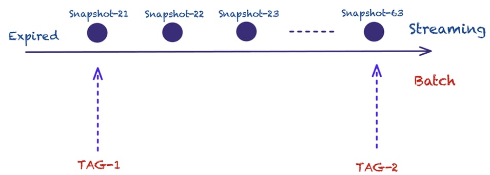
Users can create tags either manually or automatically.

In order to create tags automatically, the user needs to specify some configuration options during the table creation process.

The following code snippet depicts a table that supports automatic tag creation, using a daily interval based on processing time. Then the user can query previous versions of the table by specifying the date.

-- Flink SQL
CREATE TABLE MyTable (
   k INT PRIMARY KEY NOT ENFORCED,
   f0 INT,
   ...
) WITH (
   'tag.automatic-creation' = 'process-time',
   'tag.creation-period' = 'daily',
   'tag.creation-delay' = '10 m',
   'tag.num-retained-max' = '90'
);

INSERT INTO MyTable SELECT * FROM KafkaTable;

-- Read latest snapshot
SELECT * FROM MyTable;

-- Read Tag snapshot
SELECT * FROM MyTable VERSION AS OF '2023-07-26';

At the same time, the user can create tags manually, running a command similar to the following code snippet, by specifying a tag name and the snapshot, based on which tag needs to be created.

./bin/flink run \
   -D execution.runtime-mode=batch \
   ./jars/paimon-flink-action-0.5.0-incubating.jar \
   create-tag \
   --warehouse file:///opt/flink/temp/paimon \
   --database default \
   --table test \
   --tag-name secondtag \
   --snapshot 2

Assuming two tags are created, firsttag and secondtag, we can query based on the tags instead of specifying a timestamp, while also getting the incremental changes between two tags.

SET 'execution.runtime-mode' = 'batch';
-- read changes from snapshot id 1L
SELECT * FROM test ORDER BY id;
SELECT * FROM test /*+ OPTIONS('scan.tag-name' = 'firsttag') */;
SELECT * FROM test /*+ OPTIONS('scan.tag-name' = 'secondtag') */;

SELECT *
FROM test /*+ OPTIONS('incremental-between' = 'firsttag,secondtag') */

One benefit of Apache Paimon compared to other table formats is the use of the LSM data structure. Due to the LSM level hierarchy, minor compaction only affects upper levels that contain the incremental data. Unless there is a huge amount of incremental data, that will affect lower-levels - which contain the large files, these files can just be reused across multiple tags. This results in lower storage requirements and thus costs.

Pattern 7: CDC Data Lake Ingestion with Schema Evolution

Change data capture is a typical pattern of data ingestion. Typical use cases include capturing changes directly with Flink CDC connectors or consuming CDC data from Kafka. Apache Paimon provides a strong integration with both. At the time of writing, it supports CDC along with automatic Schema Evolution handling for MySQL, MongoDB, and Apache Kafka (with Postgres and Apache Pulsar coming in the next releases).

For Kafka, it allows integrating many different formats Canal, Debezium, Maxwell, and OGG.

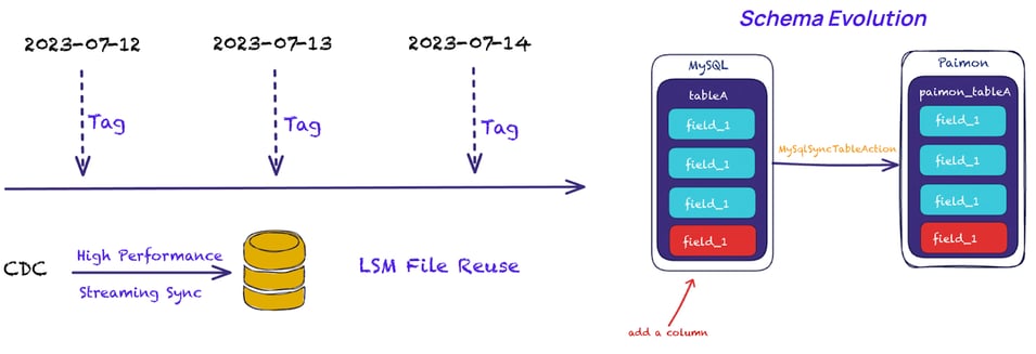
Users can also integrate with other CDC source systems by leveraging the RichCdcRecord class.

Pattern 8: Data Enrichment with Lookup Joins

Data Enrichment is another popular pattern in Stream Processing. Paimon supports Lookup joins and requires one table to have a processing time attribute. Paimon builds a Rocksdb index for Lookup Joins, which has better performance than Flink’s state.

Paimon also supports async lookups. Since we are dealing with streaming data and, in many cases, some records in the lookup table might be late to arrive, it allows using retries to account for these scenarios.

The following code snippet shows how you can perform an async lookup joins along with retries:

-- enrich each order with customer information
SELECT /*+ LOOKUP(
        'table'='c',
        'retry-predicate'='lookup_miss',
        'output-mode'='allow_unordered',
        'retry-strategy'='fixed_delay',
        'fixed-delay'='1s',
        'max-attempts'='600'
        ) */
   o.order_id, o.total, c.country, c.zip
FROM Orders AS o
        JOIN customers /*+ OPTIONS(
                         'lookup.async'='true',
                         'lookup.async-thread-number'='16'
                         ) */
   FOR SYSTEM_TIME AS OF o.proc_time AS c
             ON o.customer_id = c.id;

Pattern 9: Scalable Table for OLAP

In Pattern 5, we discussed how Paimon’s append-only table can implement message queue functionality. This is ideal for scenarios that require append-only log ingestion and implement message queue functionality.

However, some use cases might require running OLAP queries on that log ingested data and replacing Hive or Iceberg-like functionality. Once more, Paimon has this covered.

By defining bucket=-1, you can use the unaware-bucket mode.

In this mode, the concept of the bucket doesn’t exist, and data will not be shuffled in buckets. >This accelerates insertion but does not guarantee ordering any more.

We regard this as a batch offline table (although we can still perform streaming reads/writes) to run OLAP queries.

The Road Ahead

As the project is growing quickly, we might soon see more patterns being added.

Some exciting features worth keeping an eye on include:

• Paimon Metrics for better visibility
• Data Lineage for Paimon Tables
• Support for Branches
• Query Service for Paimon
• Foreign Key-based Joins

A complete list of the Paimon Improvement Proposals (PIPs) can be found here.

Conclusion

In this blog post, we explained that Apache Paimon is more than a table format. It allows the implementation of stream processing directly on the data lake. We hope that taking a pattern-based approach helps users better understand what business use cases Apache Flink and Apache Paimon help to implement directly on the data lake.

We also explored Streamhouse, which is the combination of Apache Flink, Flink CDC, and Paimon and provides the foundation that allows the extension of stream processing on the data lake when sub-second latency (like processing events directly from Kafka) is not required by the business.

The end result is significant cost reduction, and more potential use cases unlocked for data teams to explore!

Get Started

Ready to get involved? Try out the project for yourself!