Building real-time data views with Streamhouse

Use Case

Imagine an e-commerce company operating globally, we want to see, in near real-time, the amount of revenue generated per country while the order management system is processing ongoing customer orders. Order data is stored in streaming sources like Kinesis or Kafka. Customer data is coming from an OLTP database like MySQL. The goal is to calculate the total amount of revenue per country in real-time, and then share this data to a visualization layer.

Solution Overview

In this blog post, we will walk you through our solution implemented in Ververica Cloud, a fully managed ultra-high performance cloud-native service for real-time data processing. In Ververica Cloud, VERA (Ververica Runtime Assembly) is our next-generation stream processing engine based on Apache Flink. It enables real-time data processing with performance 2x better than Apache Flink. The included Flink CDC supports processing Change-Data-Capture streams out of the box. The Apache Paimon table format integrated in Ververica Cloud enables the use of cheap storage like S3 or similar and brings features of the data warehouses on top of it, such as ACID transactions, row upserts, data cataloging, time traveling, and more. In this Streamhouse, we will use VERA and Flink CDC to ingest data into Paimon and process them, then show the real-time view in a visualization layer. 

Because Paimon is the foundation for building the Streamhouse architecture, I sometimes use the terms Paimon and Streamhouse interchangeably.

High-Level Data Pipeline Design

Let's walk through how you can build this pipeline in three stages.

1. Ingestion - bring in data from different sources into the Streamhouse environment.
2. Aggregation - build data tables to share with your target users.
3. Visualization - present the data in an easy-to-read format to your users.

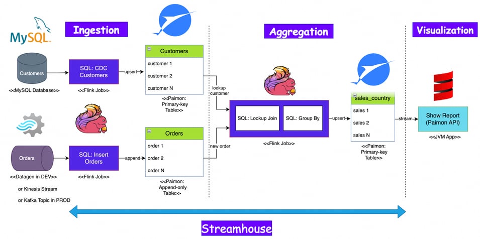
Figure 1. End-to-end data flow in Streamhouse.

As shown in the diagram, the ingestion stage includes collecting the customer order data from the MySQL database, generating the customer data using a Flink job, and then creating Paimon tables to store the data. The customer data is coming in a streaming way using Flink Change-Data-Capture(CDC). This is a crucial feature to implement an end-to-end streaming pipeline even consuming data from relational databases like MySQL. After ingesting the data, a Flink job joins two source tables and calculates the revenue per country and then builds a Paimon output table. Lastly, the Paimon Java API creates a graph to visualize the results. As the entire pipeline runs in streaming mode, there is no need to schedule some jobs recurrently, i.e. there are no batch jobs needed.

The rest of this blog provides example code for how to do this.

Create Paimon Catalog

Go to SQL Editor in Ververica Cloud, create a new SQL draft with the following SQL script to create Paimon catalog and orders table:

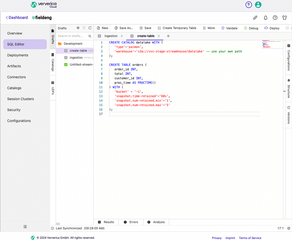
Figure 2. SQL Script to create a Paimon catalog and one table.

Ingestion

Ingestion into the streamhouse could be done by the Flink “filesystem” sink connector. However, a set of stored files alone does not give the required properties needed to build a streamhouse architecture. The right storage format for streaming data has been an issue for a long time - until Apache Paimon was created. Paimon is fully integrated in Ververica Cloud. It brings completely new opportunities to the stream processing world.

Please note that the ingestion layer stores data that can be reused for multiple purposes, so that we just copy the data as is.

Customer Order Data

Go to SQL Editor in Ververica Cloud, create a new SQL draft with the following SQL script to implement the “orders” table data ingestion:

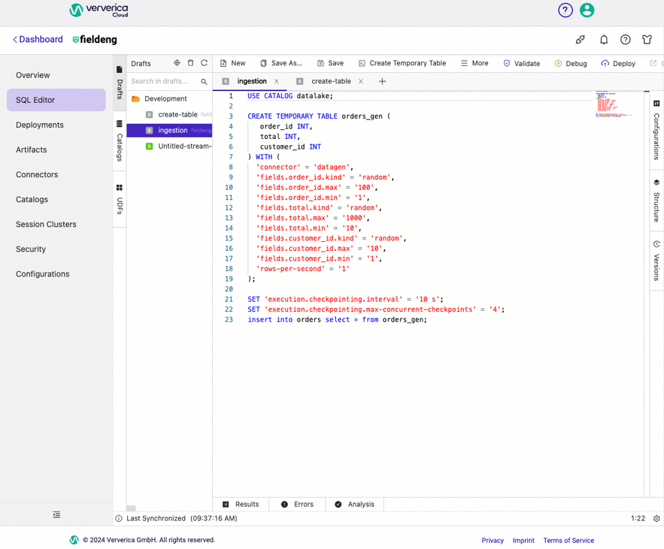
Figure 3. SQL Script to insert data into the “orders” table.

You can find full source code for ingestion in this file: https://github.com/ververica/lab-paimon-analytics/blob/main/flink-sql/ingestion.sql

Then click Deploy at the top right corner and confirm deployment:

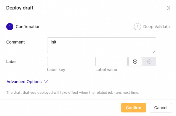
Click Deployments in the main left menu and then start your just created deployment:

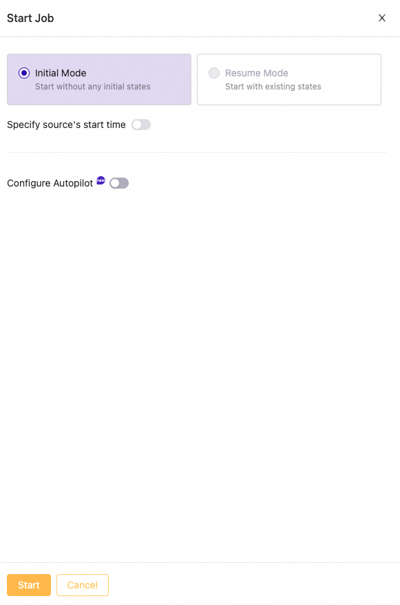
Figure 4. Start job pop-up window.

Flink SQL job results in the following Flink job graph:

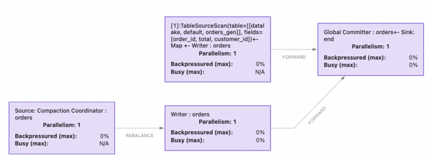
Figure 5. Flink job graph to ingest order data.

The Orders table inherits the catalog’s configuration and has its own special configuration. Bucket “-1” makes writing to this table by using a single bucket on the file storage as well as skipping data ordering guarantees. This makes writing more efficient. Using this table type works for our use case since our goal is to ingest orders into a streamhouse as fast as possible. Also, this table is set to Append Only Mode for Scale; it does not have a primary key. Since we do not need to control order_id uniqueness for our use case, we let the datagen connector generate these ids within the fixed small range.

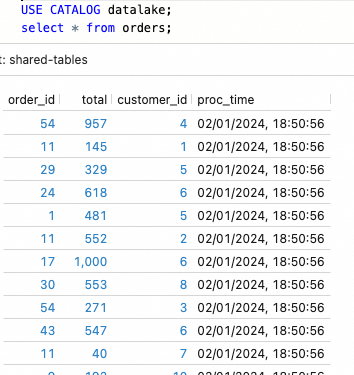
Figure 6. Data sample from the Paimon table “orders”.

Other “orders” table properties include a configuration for the file compaction process, which is done by the Paimon writer automatically. You can see an example of this on the Flink job graph as Compaction Coordinator Source. The Paimon table may create many small files which need to be periodically compacted to achieve adequate query performance.

Customer Data

This table is coming from the MySQL database. In order to prepare some data, we will use an auxiliary Flink SQL job to generate it.

This is the SQL code for the Flink Job to generate data for the customers table in MySQL database:

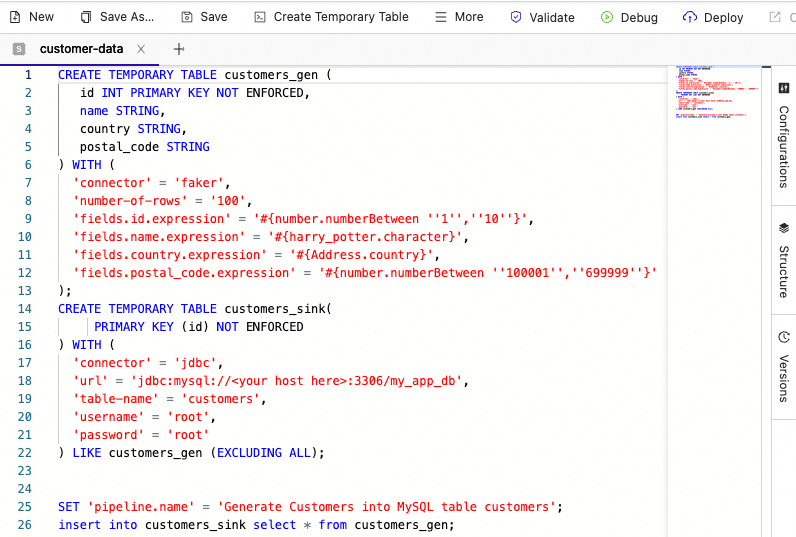
Figure 7. Data sample from the Paimon table “orders”.

Use the above SQL code to create a new Deployment in VVC and then start it.

Next, create the Paimon “customers” table to store data from the MySQL database into our Streamhouse catalog:

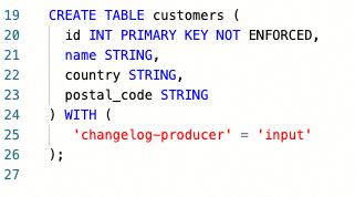
Figure 8. SQL Code to create a customer table.

There is an important setting set for the Paimon table to generate changelog files through the “input” source, as we are going to use this table later in the Lookup Join query. The “Input” producer type in our particular case relies on the change log data coming from the CDC connector, so we just reuse the input-based change log. For more information about Changelog Producers, see this page in the Paimon documentation.

To execute a CDC action to copy data into the Streamhouse, launch a Flink job with the following parameters:

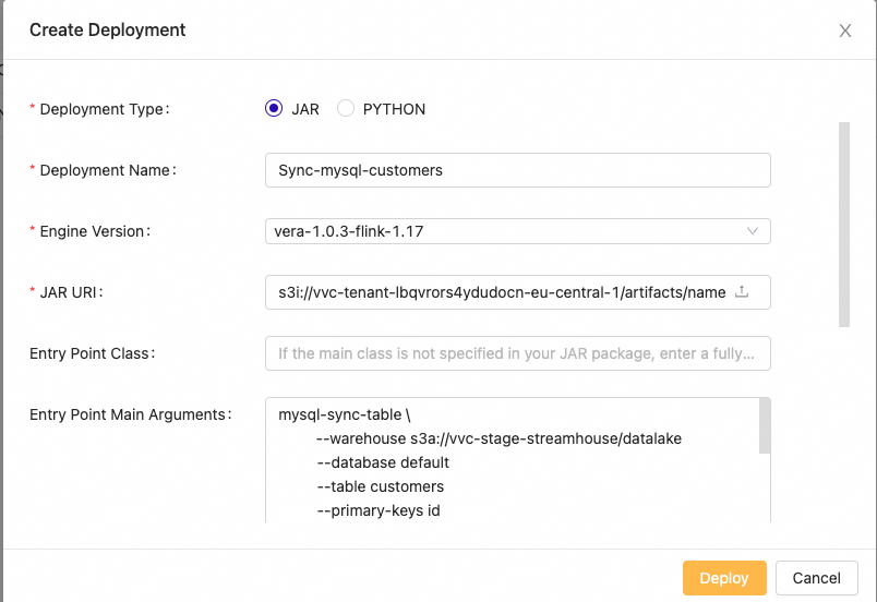
Figure 9. Deploy Paimon CDC action via JAR type deployment.

The same parameters in text can be found in the Makefile.

Once new deployment is created, go to Deployments and change this deployment configuration by setting “Checkpoint interval” to 10 seconds.

Figure 10. Change Deployment configuration.

The launch configuration above results in the following Flink job graph:

If we query the Paimon customers table, the following data displays:

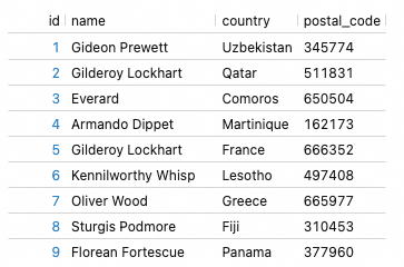
Figure 11. Data sample from the Paimon table “customers”.

Please note, the generated country names will mostly likely be different in your try

Aggregation

After ingesting the data, the next step is to use our data to start performing various aggregations, data cleaning, filtering, and building different data views for downstream users. In this example, we will join two source tables to calculate the revenue per country and store the results in another Paimon output table.

Firstly, create table by running below code in any SQL Editor window:

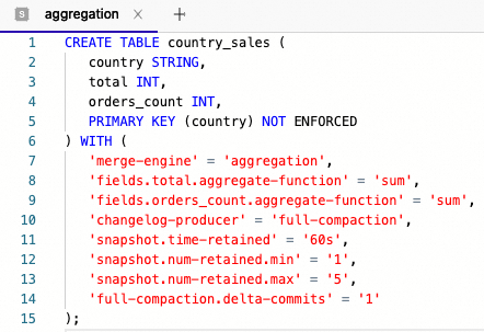
Similarly showed before, create another Flink SQL job in Ververica Cloud with the following Flink SQL code to get the revenue per country:

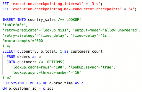
Full source code can be found here: https://github.com/ververica/lab-paimon-analytics/blob/main/flink-sql/aggregation.sql

Let’s break down the code snippets above.

First, the primary-key table uses “country” as the natural primary key with the following settings

• merge-engine=aggregation is set to automatically aggregate newly inserted records using the aggregate function’s “sum” (defined separately).
• changelog-producer=full-compaction is set to produce change log files and automatically compact them when writers insert new data into the table.
• snapshot.* properties are set to control how the compaction should work.

Next, the INSERT query is configured with SQL hints to control how the lookup should work:

• LOOKUP hint is used to retry data read if there are missing records from the customers table.
• OPTIONS hint is setting dynamic options to cache looked-up rows from customers. Also, the look-up operation is set to run in asynchronous mode not to block the entire Flink job. More on this here: https://paimon.apache.org/docs/master/how-to/lookup-joins/#async-retry-lookup
• FOR SYSTEM AS OF is used to look up customers at the point of time of a specific order processing time. This logic is important for our example but can be unnecessary for another use case, where the latest customer version should be used regardless of the order processing time.

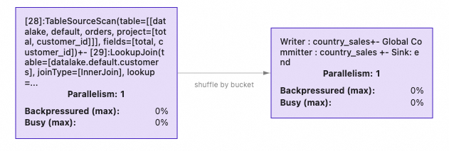
The INSERT query produces the following Flink job graph:

Visualization

Now that we have the target data, our goal is almost achieved. The remaining step is to visualize the resulting table for the end users so that they can see the revenue in real-time.

One of the standard ways to show this data to users is to use a business intelligence tool like Tableau, Power BI, or another similar tool. In order to read the Paimon table, you can either add integration with Paimon to those BI tools or come up with a way to share Paimon data in a format which those tools already support. For example, a set of JSON files can be exported and then read by Tableau.

Other users may prefer to visualize data in real-time using their web application. Paimon already has a solution for that, which is the Paimon Java API. You can build a JVM-based backend which would provide an HTTP endpoint to pull the current table into a Web UI. Moreover, using web-sockets you can also stream updates from the Paimon table on your backend service continuously to the web-socket client.

Below, you will find a Scala script which uses Paimon Java API to stream-read a Paimon table and print current table rows continuously into the console.

https://github.com/ververica/lab-paimon-analytics/blob/main/readStream.sc

You can use Ammonite script-launcher to execute this script via such command:

> amm readStream.sc

Approximately every 6 seconds (2 secs - script scan interval + 3 secs - Flink Job checkpoint) it prints country_sales table below:

We finished the implementation. Every new order produces updates to the resulting country_sales table, and every update to the customer MySQL table makes updates to the resulting view.

Customer Table Changes

Let’s make a test to see what happens if we change the country name for one of the existing customers in the MySQL table:

mysql> update customers set country = 'China' where id = 7;
Query OK, 1 row affected (0.02 sec)
Rows matched: 1  Changed: 1  Warnings: 0

You can see that a new row was inserted for ‘China’ with 4 orders and a total of 1815 revenue. The data was streamed and shown automatically from the country_sales table.

Note that the previous country name for the customer with 7 was France and it’s still there in the resulting table. If you want to see only the current countries in the customers table, then you can remove rows from the country_sales by using the Paimon Merge action.

It is currently available as a Flink DataStream batch job which can be executed as new VVC Deployment:

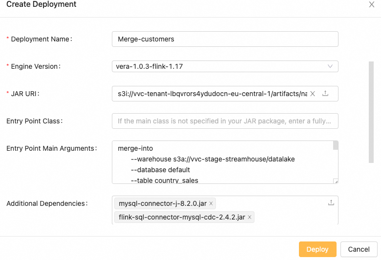
Figure 12. Merge Action Creation.

Do not forget to set Checkpoint Interval before starting the deployment:

The main logic of the Paimon action above is to merge the customers table into the country_sales table by:

1. Inserting a new country with 0 revenue in the country_sales table
2. Deleting the country from the country_sales table

For example, ‘France’ no longer occurs in the customer table, so it is going to be deleted from country_sales after the merge action is executed.

Before executing this Paimon action, let’s also add a new customer with a new id and a new country name which is not already used by the order data generation job. This allows us to get a new country name with 0 revenue in the country_sales table:

mysql> insert into customers values(11, 'Santa', 'North Pole', '000001');
Query OK, 1 row affected (0.01 sec)

Now you can run the merge action.

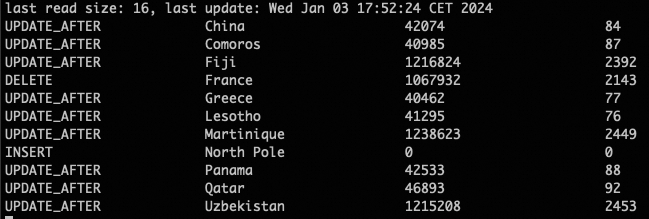
After the merge, you can see the expected outcome:

1. Country name ‘France’ and its row is removed
2. Country name ‘North Pole’ (fictional) is added with 0 revenue

By doing it this way, we synced the customers table with the country_sales table without using the orders table.

What Apache Paimon unlocks for Data Teams

You no longer need a compute-expensive data storage system like Apache Kafka (or similar) to apply stream processing while working with intermediate data sets. This can be achieved by using Paimon “Append Only” tables. They allow replacing message queues for data ingestion to the streamhouse. This is of course, only applicable if you can tolerate data delays which depend on Flink checkpoint interval (it is configurable).

Paimon treats Flink as the reference implementation of the stream processing framework and supports core Flink functionality for streaming and batch data processing. Storing data in Paimon tables allows you to leverage cheap storage services like S3 and at the same time you get the main OLAP/data warehouse properties, which are crucial to implement data analytics and machine learning applications on top of the streamhouse.

Interested? Then give a try in Ververica Cloud to implement your own Streamhouse. If you sign up for the first time, you can get a $400 credit to start.